pacman::p_load(sf,spdep, tmap, tidyverse,dplyr, funModeling,rgdal, ClustGeo, ggpubr, cluster, factoextra, NbClust,heatmaply, corrplot, psych, GGally)Take-home Exercise 2: Regionalisation of Multivariate Water Point Attributes with Non-spatially Constrained and Spatially Constrained Clustering Methods
1 Getting Started
2 Data Import
Import water point data
wp <- read_csv("Take home 2 data/WPdx.csv",show_col_types = FALSE) %>%
  filter(`#clean_country_name` == "Nigeria")
I use
show_col_types = FALSEto avoid warning message.To extract Nigeria data I use
filter()
wp_nga <- read_rds("Take home 2 data/wp_nga.rds") wp_nga <- wp_nga %>%
select(`lat_deg`, `lon_deg`, `X_water_tec`, `clean_adm2`, `status_cle`, `usage_cap`, `is_urban`,`geometry`)write_rds(wp_nga,"Take home 2 data/wp_nga mini.rds")wp_nga <- read_rds("Take home 2 data/wp_nga mini.rds") Convert wkt data
Column ‘New Georaferenced Column’ represent spatial data in a textual format. this kind of text file is popularly known as Well Known Text in short wkt.
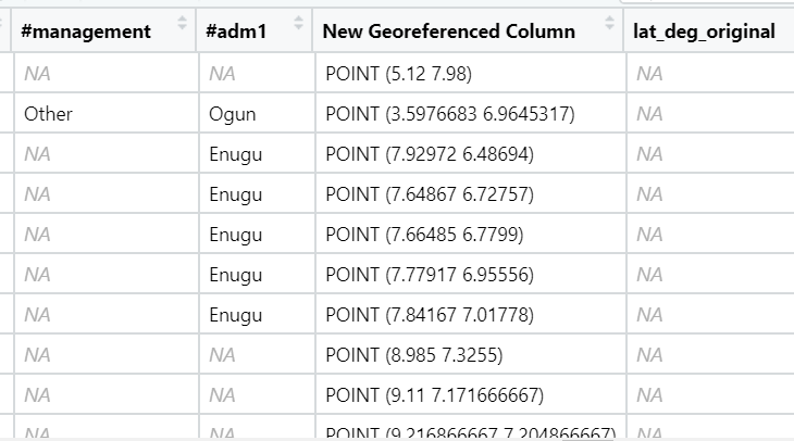
Two steps will be used to convert an asptial data file in wkt format into a sf data frame by using sf.
First, st_as_sfc() of sf package is used to derive a new field called Geometry as shown in the code chunk below.
wp_nga$Geometry = st_as_sfc(wp_nga$`New Georeferenced Column`)Now we get the new column called Geometry.
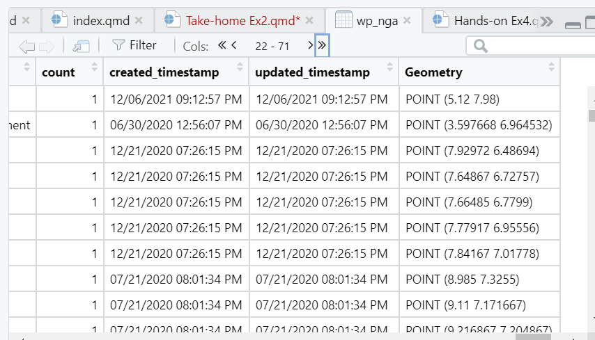
Next, st_sf() will be used to convert the tibble data frame into sf data frame.
wp_sf <- st_sf(wp_nga, crs=4326) When the process completed, a new sf data frame called wp_sf will be created.
Importing Nigeria LGA level boundary data
nga<- st_read(dsn="Take home 2 data",
             layer="geoBoundaries-NGA-ADM2",
             crs=4326)
Reading layer `geoBoundaries-NGA-ADM2' from data source
`D:\Xu-Siyi\ISSS624\Take-home Exercise\Take home 2 data' using driver `ESRI Shapefile'
Simple feature collection with 774 features and 5 fields
Geometry type: MULTIPOLYGON
Dimension: XY
Bounding box: xmin: 2.668534 ymin: 4.273007 xmax: 14.67882 ymax: 13.89442
Geodetic CRS: WGS 84Point in Polygon Overlay
To make sure the data accuracy, we are going to use a geoprocessing function (or commonly know as GIS analysis) called point-in-polygon overlay to transfer the attribute information in nga sf data frame into wp_sf data frame.
wp_sf <- st_join(wp_sf, nga)%>%
  mutate(status_cle = replace_na(status_cle, "Unknown")) %>%
  mutate(X_water_tec = replace_na(X_water_tec, "Unknown"))
Now we have column called “shapeName”, which is the LGA name of Nigeria water point.

3 Data Wrangling
The reference of the code chunk in Data Wrangling part: Ong Zhi Rong Jordan
Checking of duplicated area name
We use duplicate function to retrieve all the shapeName that has duplicates and store it in a list. From the result below, we identified 12 shapeNames that are duplicates.
nga <- (nga[order(nga$shapeName), ])

duplicate_area <- nga$shapeName[ nga$shapeName %in% nga$shapeName[duplicated(nga$shapeName)] ]

duplicate_area
[1] "Bassa" "Bassa" "Ifelodun" "Ifelodun" "Irepodun" "Irepodun"
[7] "Nasarawa" "Nasarawa" "Obi" "Obi" "Surulere" "Surulere"Next, we will leverage on the interactive viewer of tmap to check the location of each area. Through the use of Google, we are able to retrieve the actual name and state of the areas. The table below shows the index and the actual name of the area.
| Index | Actual Area Name |
|---|---|
| 94 | Bassa (Kogi) |
| 95 | Bassa (Plateau) |
| 304 | Ifelodun (Kwara) |
| 305 | Ifelodun (Osun) |
| 355 | Irepodun (Kwara) |
| 356 | Irepodun (Osun) |
| 518 | Nassarawa |
| 546 | Obi (Benue) |
| 547 | Obi(Nasarawa) |
| 693 | Surulere (lagos) |
| 694 | Surulere (Oyo) |
tmap_mode("view")tmap mode set to interactive viewingtm_shape(nga[nga$shapeName %in% duplicate_area,]) +
tm_polygons()Make sure the tmap mode set back to plot
tmap_mode("plot")tmap mode set to plottingWe will now access the individual index of the nga data frame and change the value. Lastly, we use the length() function to ensure there is no more duplicated shapeName.
nga$shapeName[c(94,95,304,305,355,356,519,546,547,693,694)] <- c("Bassa (Kogi)","Bassa (Plateau)",
                                                                               "Ifelodun (Kwara)","Ifelodun (Osun)",
                                                                               "Irepodun (Kwara)","Irepodun (Osun)",
                                                                               "Nassarawa","Obi (Benue)","Obi(Nasarawa)",
                                                                               "Surulere (Lagos)","Surulere (Oyo)")

length((nga$shapeName[ nga$shapeName %in% nga$shapeName[duplicated(nga$shapeName)] ]))
[1] 0Projection of sf dataframe
wp_sf <- st_as_sf(nga, coords = c("long", "lat"), crs = 4326)4 Derive new variables
Take-home Exercise 2 Objective
In this take-home exercise you are required to regionalise Nigeria by using, but not limited to the following measures:
Total number of functional water points
Total number of nonfunctional water points
Percentage of functional water points
Percentage of non-functional water points
Percentage of main water point technology (i.e. Hand Pump)
Percentage of usage capacity (i.e. < 1000, >=1000)
Percentage of rural water points
In this section, we will extract the water point records by using classes in status_cle field.
in this code chunk below, filter() is used to select functional water points
wpt_functional <- wp_sf %>%
  filter(status_cle %in%
           c("Functional",
             "Functional but not in use",
             "Functional but needs repair"))
In the code chunk below, filter() of dplyr is used to select non-functional water points.
wpt_nonfunctional <- wp_sf %>%
  filter(status_cle %in%
           c("Abandoned/Decommissioned",
             "Abandoned",
             "Non-Functional",
             "Non functional due to dry season",
             "Non-Functional due to dry season"))
In the code chunk below, filter() of dplyr is used to select water points with unknown status.
wpt_unknown <- wp_sf %>%
  filter(status_cle == "Unknown")
wpt_handpump <- wp_sf %>%
filter(X_water_tec == "Hand Pump")usage_low <- wp_sf %>%
filter(`usage_cap` < 1000)usage_high <- wp_sf %>%
filter(`usage_cap` >= 1000)wpt_rural<-wp_sf %>%
filter(`is_urban` == "False")Then we add new variable called total wpt, wpt functional, wpt non-functional, wpt unknown, wpt handpump, usage low, usage high, `wpt rural into nga dataframe.
nga_wp <- nga %>%
  mutate(`total wpt` = lengths(
    st_intersects(nga, wp_sf))) %>%
  mutate(`wpt functional` = lengths(
    st_intersects(nga, wpt_functional))) %>%
  mutate(`wpt non-functional` = lengths(
    st_intersects(nga, wpt_nonfunctional))) %>%
  mutate(`wpt unknown` = lengths(
    st_intersects(nga, wpt_unknown)))%>%
  mutate(`wpt handpump` = lengths(
    st_intersects(nga, wpt_handpump)))%>%
  mutate(`usage low` = lengths(
    st_intersects(nga, usage_low)))%>%
  mutate(`usage high` = lengths(
    st_intersects(nga, usage_high)))%>%
  mutate(`wpt rural` = lengths(
    st_intersects(nga, wpt_rural)))
Then we can calculate the percentage of functional water point and non-functional water points, the percentage of Hand Pump, the percentage of usage capacity and the percentage of rural water points
nga_wp <- nga_wp %>%
  mutate(pct_functional = `wpt functional`/`total wpt`) %>%
  mutate(`pct_non-functional` = `wpt non-functional`/`total wpt`) %>%
  mutate(`pct_handpump` = `wpt handpump`/`total wpt`) %>%
  mutate(`pct_usagelow` = `usage low`/`total wpt`) %>%
  mutate(`pct_usagehigh` = `usage high`/`total wpt`) %>%
  mutate(`pct_rural` = `wpt rural`/`total wpt`)
Things to learn from the code chunk above:
mutate() of dplyr package is used to derive two fields namely pct_functional and pct_non-functional.
There are some NaN field in the nga_wp because of the zero number of total water point. I replace them with zero value.
nga_wp <- nga_wp %>%
  mutate(pct_functional = replace_na(pct_functional, 0)) %>%
  mutate(`pct_non-functional` = replace_na(`pct_non-functional`, 0)) %>%
  mutate(pct_handpump = replace_na(pct_handpump, 0)) %>%
  mutate(pct_usagelow = replace_na(pct_usagelow, 0)) %>%
  mutate(pct_usagehigh = replace_na(pct_usagehigh, 0)) %>%
  mutate(pct_rural = replace_na(pct_rural, 0))
wp_sf <- st_transform(wp_sf, crs = 26391)
st_crs (wp_sf)Coordinate Reference System:
User input: EPSG:26391
wkt:
PROJCRS["Minna / Nigeria West Belt",
BASEGEOGCRS["Minna",
DATUM["Minna",
ELLIPSOID["Clarke 1880 (RGS)",6378249.145,293.465,
LENGTHUNIT["metre",1]]],
PRIMEM["Greenwich",0,
ANGLEUNIT["degree",0.0174532925199433]],
ID["EPSG",4263]],
CONVERSION["Nigeria West Belt",
METHOD["Transverse Mercator",
ID["EPSG",9807]],
PARAMETER["Latitude of natural origin",4,
ANGLEUNIT["degree",0.0174532925199433],
ID["EPSG",8801]],
PARAMETER["Longitude of natural origin",4.5,
ANGLEUNIT["degree",0.0174532925199433],
ID["EPSG",8802]],
PARAMETER["Scale factor at natural origin",0.99975,
SCALEUNIT["unity",1],
ID["EPSG",8805]],
PARAMETER["False easting",230738.26,
LENGTHUNIT["metre",1],
ID["EPSG",8806]],
PARAMETER["False northing",0,
LENGTHUNIT["metre",1],
ID["EPSG",8807]]],
CS[Cartesian,2],
AXIS["(E)",east,
ORDER[1],
LENGTHUNIT["metre",1]],
AXIS["(N)",north,
ORDER[2],
LENGTHUNIT["metre",1]],
USAGE[
SCOPE["Engineering survey, topographic mapping."],
AREA["Nigeria - onshore west of 6°30'E, onshore and offshore shelf."],
BBOX[3.57,2.69,13.9,6.5]],
ID["EPSG",26391]]Now, I have the tidy sf data table subsequent analysis and save the sf data table into rds format. nga_wp.rds, which is the combination of the geospatial and aspatial data.
write_rds(nga_wp, "Take home 2 data/nga_wp.rds")
write_rds(wp_sf, "Take home 2 data/wp_sf.rds")
5 Exploratory Data Analysis (EDA)
nga_wp <- read_rds("Take home 2 data/nga_wp.rds")
wp_sf <- read_rds("Take home 2 data/wp_sf.rds")
EDA using statistical graphics
Firstly, I plot the distribution of the variables (i.e. Number of functional water point) by using bar graph.
freq(data=wp_sf,
     input = 'status_cle')
Warning: The `<scale>` argument of `guides()` cannot be `FALSE`. Use "none" instead as
of ggplot2 3.3.4.
ℹ The deprecated feature was likely used in the funModeling package.
Please report the issue at <https://github.com/pablo14/funModeling/issues>.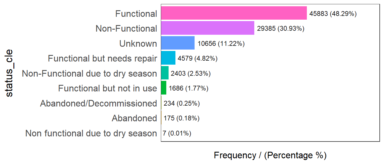
                        status_cle frequency percentage cumulative_perc
1                       Functional     45883      48.29           48.29
2                   Non-Functional     29385      30.93           79.22
3                          Unknown     10656      11.22           90.44
4      Functional but needs repair      4579       4.82           95.26
5 Non-Functional due to dry season      2403       2.53           97.79
6        Functional but not in use      1686       1.77           99.56
7         Abandoned/Decommissioned       234       0.25           99.81
8                        Abandoned       175       0.18           99.99
9 Non functional due to dry season         7       0.01          100.00
From the graph above we can see there are 48.29% water points in Nigeria are functional. 30.93% water points are non-functional and 11.22% water points are unknown.
freq(data=wp_sf,
     input = 'X_water_tec')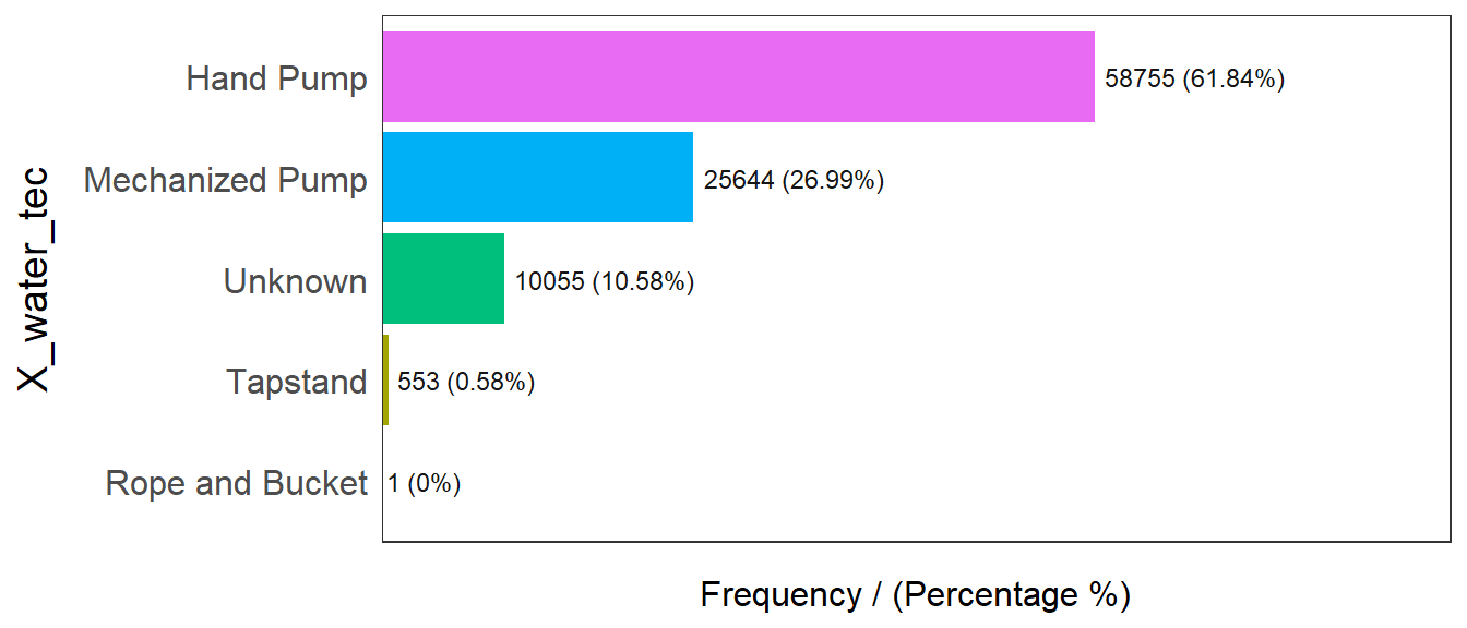
      X_water_tec frequency percentage cumulative_perc
1       Hand Pump     58755      61.84           61.84
2 Mechanized Pump     25644      26.99           88.83
3         Unknown     10055      10.58           99.41
4        Tapstand       553       0.58           99.99
5 Rope and Bucket         1       0.00          100.00
From the above graph we can see that 61.84% of all water points in Nigeria are hand pump, 26.99% are mechanized pump and 10.58% are unknown.
freq(data=wp_sf,
     input = 'is_urban')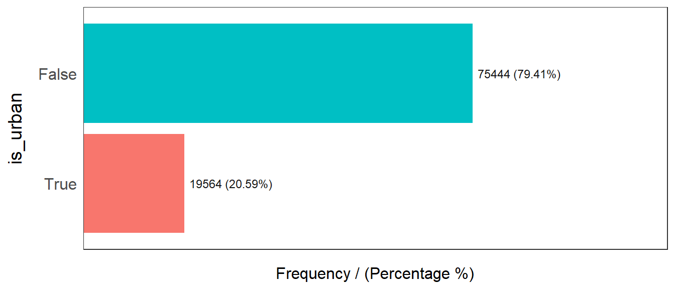
  is_urban frequency percentage cumulative_perc
1    False     75444      79.41           79.41
2     True     19564      20.59          100.00
From the above graph we can see that 79.14% of all water points in Nigeria are rural, 20.59% are urban.
Secondly, I plot the distribution of the variables (i.e. Number of functional water point) by using historgram graph.
pct_functional <- ggplot(data=nga_wp,
             aes(x= `pct_functional`)) +
  geom_histogram(bins=20,
                 color="black",
                 fill="light blue")

pct_nonfunctional <- ggplot(data=nga_wp,
             aes(x= `pct_non-functional`)) +
  geom_histogram(bins=20,
                 color="black",
                 fill="light blue")

pct_handpump <- ggplot(data=nga_wp,
           aes(x= `pct_handpump`)) +
geom_histogram(bins=20,
               color="black",
                 fill="light blue")

pct_usagelow <- ggplot(data=nga_wp,
             aes(x= `pct_usagelow`)) +
  geom_histogram(bins=20,
                 color="black",
                 fill="light blue")

pct_usagehigh <- ggplot(data=nga_wp,
             aes(x= `pct_usagehigh`)) +
  geom_histogram(bins=20,
                 color="black",
                 fill="light blue")

pct_rural <- ggplot(data=nga_wp,
             aes(x= `pct_rural`)) +
  geom_histogram(bins=20,
                 color="black",
fill="light blue")ggarrange(pct_functional, pct_nonfunctional,pct_handpump, pct_usagehigh, pct_usagelow, pct_rural,
ncol = 3,
nrow = 2)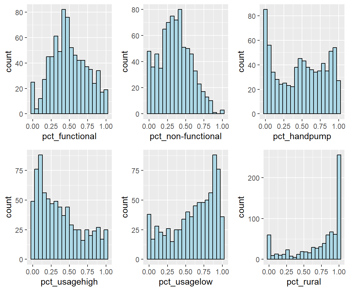
EDA using choropleth map
I prepared a choropleth map to have a quick look at the distribution of water point in Nigeria
The code chunks below are used to prepare the choroplethby using the qtm() function of tmap package.
qtm(nga_wp, "total wpt")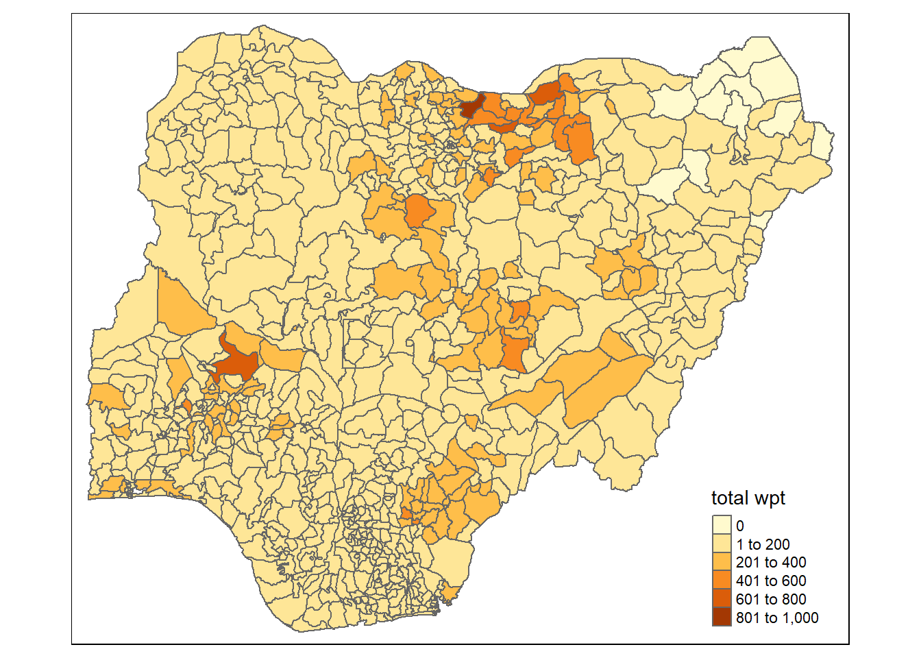
func.map <- tm_shape(nga_wp) +
  tm_fill(col = "pct_functional",
          n = 5,
          style = "jenks") +
  tm_borders(alpha = 0.5)

nonfunc.map <- tm_shape(nga_wp) +
  tm_fill(col = "pct_non-functional",
          n = 5,
          style = "jenks") +
  tm_borders(alpha = 0.5)

handpump.map <- tm_shape(nga_wp) +
  tm_fill(col = "pct_handpump",
          n = 5,
          style = "jenks") +
  tm_borders(alpha = 0.5)

usagelow.map <- tm_shape(nga_wp) +
  tm_fill(col = "pct_usagelow",
          n = 5,
          style = "jenks") +
  tm_borders(alpha = 0.5)

usagehigh.map <- tm_shape(nga_wp) +
  tm_fill(col = "pct_usagehigh",
          n = 5,
          style = "jenks") +
  tm_borders(alpha = 0.5)

rural.map <- tm_shape(nga_wp) +
  tm_fill(col = "pct_rural",
          n = 5,
          style = "jenks") +
  tm_borders(alpha = 0.5)

tmap_arrange(func.map, nonfunc.map,handpump.map,usagelow.map,usagehigh.map,rural.map,
             asp=NA, ncol=2)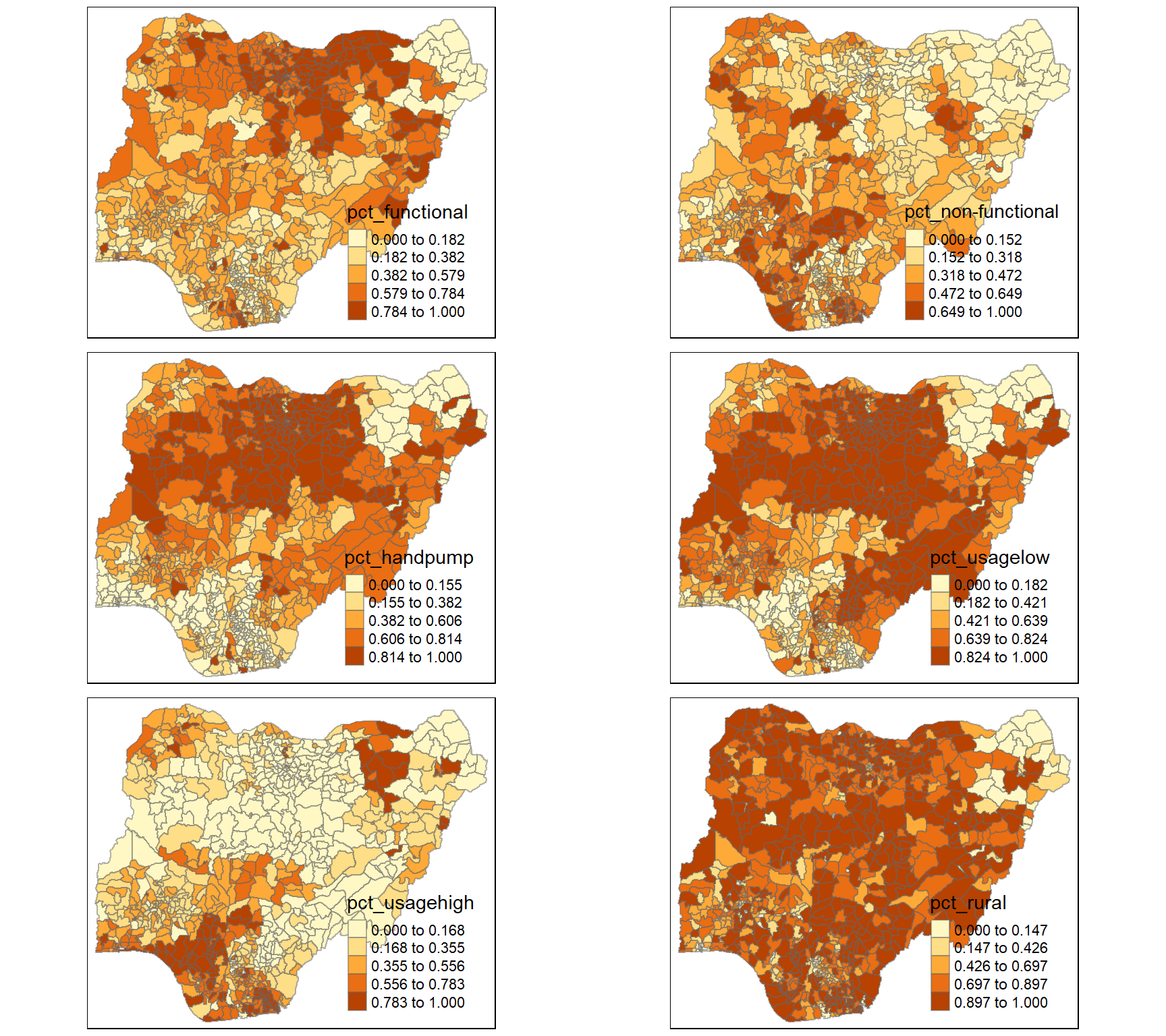
6 Correlation Analysis
nga_wp_cor <- nga_wp %>%
  st_drop_geometry() %>%
  select("shapeName","wpt functional","wpt non-functional", "pct_functional", "pct_non-functional", "pct_handpump","pct_usagelow","pct_usagehigh", "pct_rural")
cluster_vars.cor = cor(nga_wp_cor[,2:8])
corrplot.mixed(cluster_vars.cor,
         lower = "ellipse",
               upper = "number",
               tl.pos = "lt",
               diag = "l",
               tl.col = "black")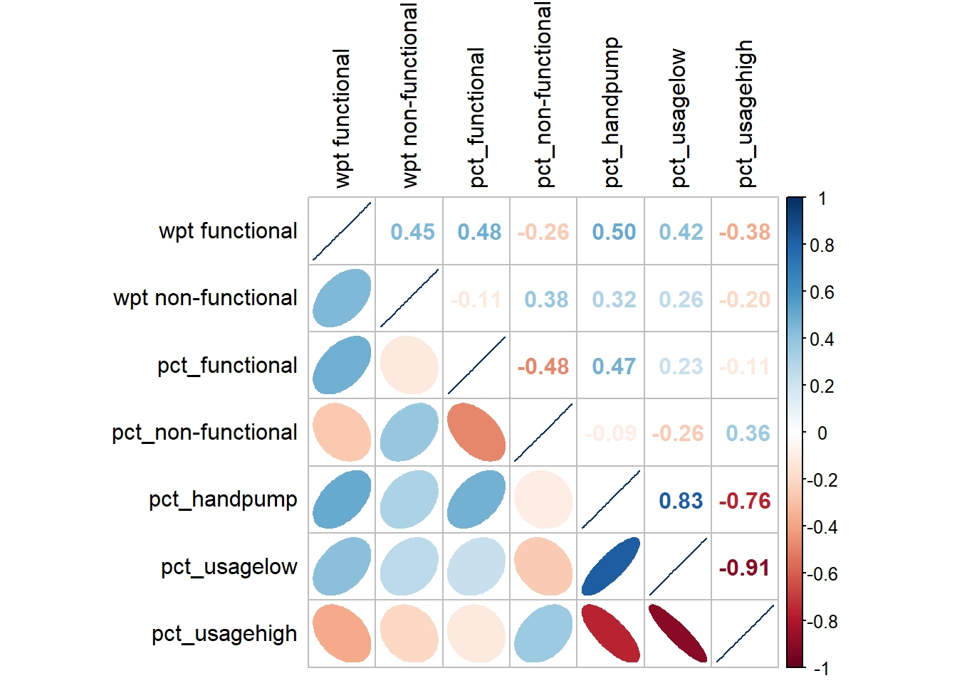
7 Hierarchy Cluster Analysis
Extracting clustering variables
cluster_vars <- nga_wp_cor %>%
  select("shapeName","wpt functional","wpt non-functional","pct_functional", "pct_non-functional", "pct_handpump","pct_usagelow","pct_usagehigh", "pct_rural")
head(cluster_vars,10)
shapeName wpt functional wpt non-functional pct_functional
1 Aba North 7 9 0.4117647
2 Aba South 29 35 0.4084507
3 Abadam 0 0 0.0000000
4 Abaji 23 34 0.4035088
5 Abak 23 25 0.4791667
6 Abakaliki 82 42 0.3519313
7 Abeokuta North 16 15 0.4705882
8 Abeokuta South 72 33 0.6050420
9 Abi 79 62 0.5197368
10 Aboh-Mbaise 18 26 0.2727273
pct_non-functional pct_handpump pct_usagelow pct_usagehigh pct_rural
1 0.5294118 0.11764706 0.17647059 0.8235294 0.00000000
2 0.4929577 0.09859155 0.12676056 0.8732394 0.05633803
3 0.0000000 0.00000000 0.00000000 0.0000000 0.00000000
4 0.5964912 0.40350877 0.40350877 0.5964912 0.84210526
5 0.5208333 0.08333333 0.08333333 0.9166667 0.83333333
6 0.1802575 0.43776824 0.90557940 0.0944206 0.87553648
7 0.4411765 0.14705882 0.23529412 0.7647059 0.20588235
8 0.2773109 0.16806723 0.29411765 0.7058824 0.00000000
9 0.4078947 0.59868421 0.67105263 0.3289474 0.95394737
10 0.3939394 0.01515152 0.34848485 0.6515152 0.72727273Next, we need to change the rows by shape name instead of row number by using the code chunk below.
row.names(cluster_vars) <- cluster_vars$"shapeName"
head(cluster_vars,10)
shapeName wpt functional wpt non-functional pct_functional
Aba North Aba North 7 9 0.4117647
Aba South Aba South 29 35 0.4084507
Abadam Abadam 0 0 0.0000000
Abaji Abaji 23 34 0.4035088
Abak Abak 23 25 0.4791667
Abakaliki Abakaliki 82 42 0.3519313
Abeokuta North Abeokuta North 16 15 0.4705882
Abeokuta South Abeokuta South 72 33 0.6050420
Abi Abi 79 62 0.5197368
Aboh-Mbaise Aboh-Mbaise 18 26 0.2727273
pct_non-functional pct_handpump pct_usagelow pct_usagehigh
Aba North 0.5294118 0.11764706 0.17647059 0.8235294
Aba South 0.4929577 0.09859155 0.12676056 0.8732394
Abadam 0.0000000 0.00000000 0.00000000 0.0000000
Abaji 0.5964912 0.40350877 0.40350877 0.5964912
Abak 0.5208333 0.08333333 0.08333333 0.9166667
Abakaliki 0.1802575 0.43776824 0.90557940 0.0944206
Abeokuta North 0.4411765 0.14705882 0.23529412 0.7647059
Abeokuta South 0.2773109 0.16806723 0.29411765 0.7058824
Abi 0.4078947 0.59868421 0.67105263 0.3289474
Aboh-Mbaise 0.3939394 0.01515152 0.34848485 0.6515152
pct_rural
Aba North 0.00000000
Aba South 0.05633803
Abadam 0.00000000
Abaji 0.84210526
Abak 0.83333333
Abakaliki 0.87553648
Abeokuta North 0.20588235
Abeokuta South 0.00000000
Abi 0.95394737
Aboh-Mbaise 0.72727273Notice that the row number has been replaced into the township name.
Now, we will delete the Shape Name field by using the code chunk below.
nga_wp_clu <- select(cluster_vars, c(2:9))
head(nga_wp_clu, 10)
wpt functional wpt non-functional pct_functional
Aba North 7 9 0.4117647
Aba South 29 35 0.4084507
Abadam 0 0 0.0000000
Abaji 23 34 0.4035088
Abak 23 25 0.4791667
Abakaliki 82 42 0.3519313
Abeokuta North 16 15 0.4705882
Abeokuta South 72 33 0.6050420
Abi 79 62 0.5197368
Aboh-Mbaise 18 26 0.2727273
pct_non-functional pct_handpump pct_usagelow pct_usagehigh
Aba North 0.5294118 0.11764706 0.17647059 0.8235294
Aba South 0.4929577 0.09859155 0.12676056 0.8732394
Abadam 0.0000000 0.00000000 0.00000000 0.0000000
Abaji 0.5964912 0.40350877 0.40350877 0.5964912
Abak 0.5208333 0.08333333 0.08333333 0.9166667
Abakaliki 0.1802575 0.43776824 0.90557940 0.0944206
Abeokuta North 0.4411765 0.14705882 0.23529412 0.7647059
Abeokuta South 0.2773109 0.16806723 0.29411765 0.7058824
Abi 0.4078947 0.59868421 0.67105263 0.3289474
Aboh-Mbaise 0.3939394 0.01515152 0.34848485 0.6515152
pct_rural
Aba North 0.00000000
Aba South 0.05633803
Abadam 0.00000000
Abaji 0.84210526
Abak 0.83333333
Abakaliki 0.87553648
Abeokuta North 0.20588235
Abeokuta South 0.00000000
Abi 0.95394737
Aboh-Mbaise 0.72727273Data Standardisation
In order to avoid the cluster analysis result is baised to clustering variables with large values, it is useful to standardise the input variables before performing cluster analysis
Min-Max standardisation
In the code chunk below, normalize() of heatmaply package is used to stadardisation the clustering variables by using Min-Max method. The summary() is then used to display the summary statistics of the standardised clustering variables.
nga_wp_clu.std <- normalize(cluster_vars)
summary(nga_wp_clu.std)
shapeName wpt functional wpt non-functional pct_functional
Length:774 Min. :0.00000 Min. :0.00000 Min. :0.0000
Class :character 1st Qu.:0.02261 1st Qu.:0.04406 1st Qu.:0.3261
Mode :character Median :0.06051 Median :0.12230 Median :0.4741
Mean :0.08957 Mean :0.14962 Mean :0.4984
3rd Qu.:0.11669 3rd Qu.:0.21853 3rd Qu.:0.6699
Max. :1.00000 Max. :1.00000 Max. :1.0000
pct_non-functional pct_handpump pct_usagelow pct_usagehigh
Min. :0.0000 Min. :0.0000 Min. :0.0000 Min. :0.0000
1st Qu.:0.2105 1st Qu.:0.1670 1st Qu.:0.3968 1st Qu.:0.1220
Median :0.3505 Median :0.5099 Median :0.6703 Median :0.3127
Mean :0.3592 Mean :0.4873 Mean :0.6078 Mean :0.3754
3rd Qu.:0.5076 3rd Qu.:0.7778 3rd Qu.:0.8735 3rd Qu.:0.5771
Max. :1.0000 Max. :1.0000 Max. :1.0000 Max. :1.0000
pct_rural
Min. :0.0000
1st Qu.:0.5727
Median :0.8645
Mean :0.7271
3rd Qu.:1.0000
Max. :1.0000 Notice that the values range of the Min-max standardised clustering variables are 0-1 now.
Z-score standardisation
Z-score standardisation can be performed easily by using scale() of Base R. The code chunk below will be used to stadardisation the clustering variables by using Z-score method.
I wont use Z score standardisation because not all variables come from normal distribution.
Visualising the standardised clustering variables
r <- ggplot(data=nga_wp,
             aes(x= `pct_functional`)) +
  geom_histogram(bins=20,
                 color="black",
                 fill="light blue") +
  ggtitle("Raw values without standardisation")

nga_clu_s_df <- as.data.frame(nga_wp_clu.std)
s <- ggplot(data=nga_clu_s_df,
       aes(x=`pct_functional`)) +
  geom_histogram(bins=20,
                 color="black",
                 fill="light blue") +
  ggtitle("Min-Max Standardisation")

ggarrange(r, s,
          ncol = 2,
          nrow = 1)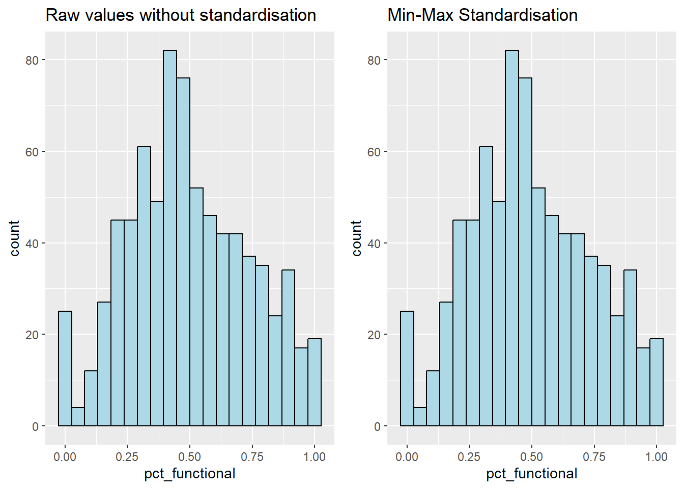
r <- ggplot(data=nga_wp,
             aes(x= `pct_functional`)) +
  geom_density(color="black",
               fill="light blue") +
  ggtitle("Raw values without standardisation")

nga_clu_s_df <- as.data.frame(nga_wp_clu.std)
s <- ggplot(data=nga_clu_s_df,
       aes(x=`pct_functional`)) +
  geom_density(color="black",
               fill="light blue") +
  ggtitle("Min-Max Standardisation")

ggarrange(r, s,
          ncol = 2,
          nrow = 1)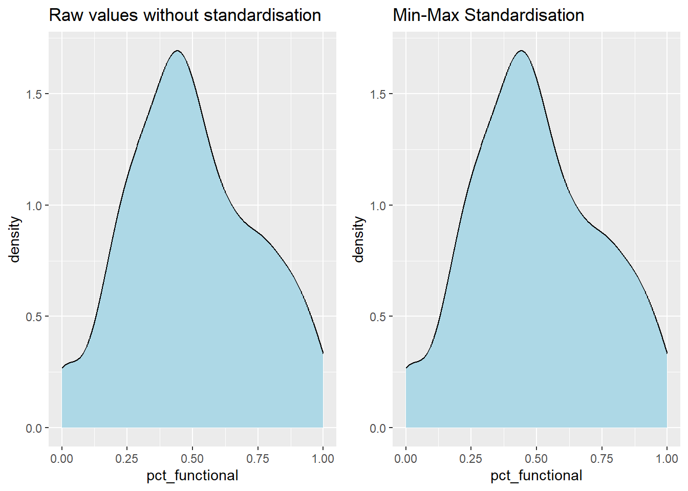
Computing proximity matrix
The code chunk below is used to compute the proximity matrix using euclidean method.
proxmat <- dist(nga_wp_clu, method = 'euclidean')The code chunk below can then be used to list the content of proxmat for visual inspection.
proxmatComputing hierarchical clustering
hclust_ward <- hclust(proxmat, method = 'ward.D')plot(hclust_ward, cex = 0.6)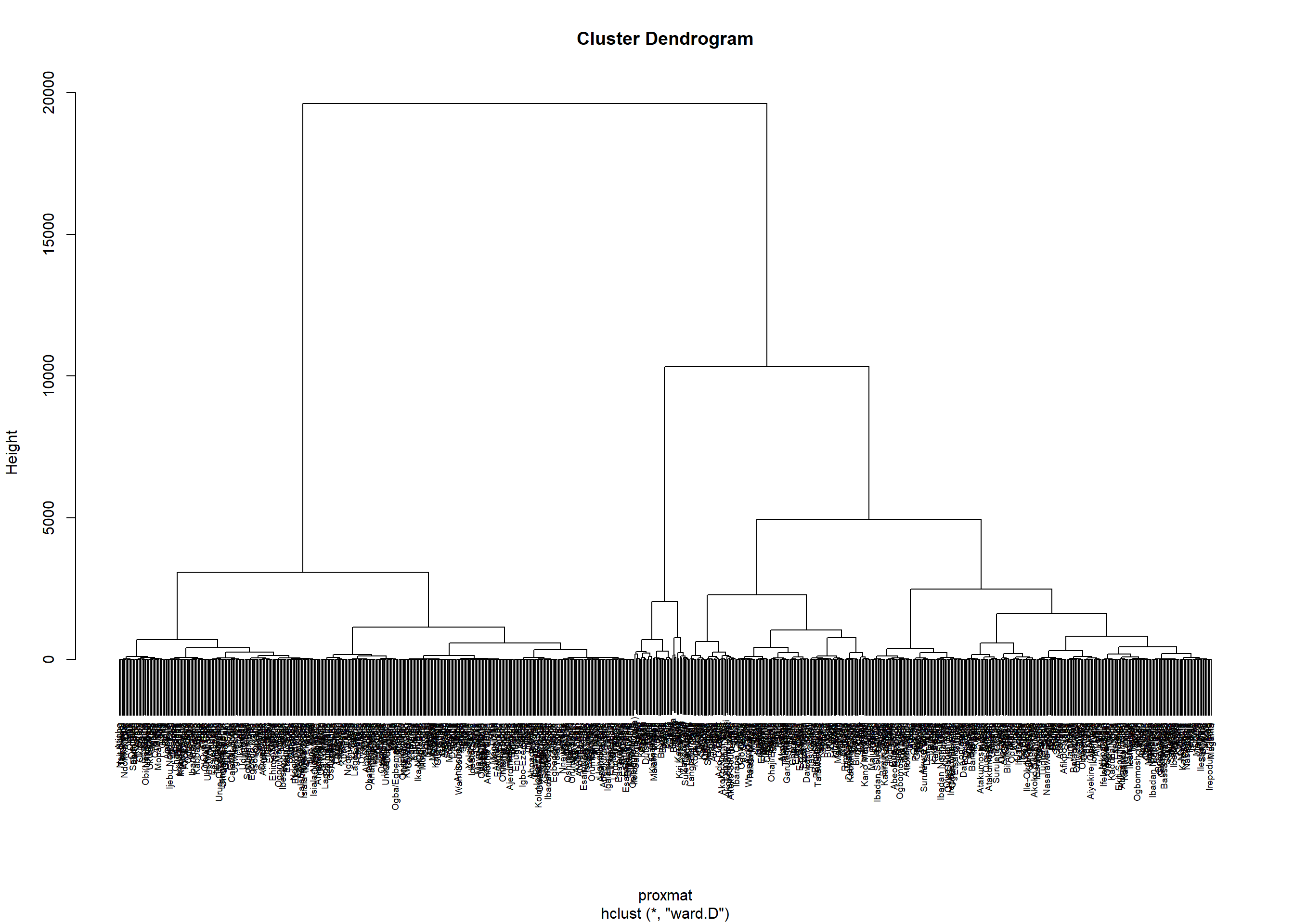
Selecting the optimal clustering algorithm
The code chunk below will be used to compute the agglomerative coefficients of all hierarchical clustering algorithms.
Values closer to 1 suggest strong clustering structure.
m <- c( "average", "single", "complete", "ward")
names(m) <- c( "average", "single", "complete", "ward")

ac <- function(x) {
  agnes(nga_wp_clu, method = x)$ac
}

map_dbl(m, ac)
average single complete ward
0.9921897 0.9697080 0.9935520 0.9980737 With reference to the output above, we can see that Ward’s method, which value=0.998 is most closer to 1 provides the strongest clustering structure among the four methods assessed. Hence, in the subsequent analysis, only Ward’s method will be used.
Determining Optimal Clusters
There are three commonly used methods to determine the optimal clusters, they are:
Elbow Method
Average Silhouette Method
Gap Statistic Method
Gap Statistic Method
set.seed(12345)
gap_stat <- clusGap(nga_wp_clu,
                    FUN = hcut,
                    nstart = 25,
                    K.max = 10,
                    B = 50)
# Print the result
print(gap_stat, method = "firstmax")
Clustering Gap statistic ["clusGap"] from call:
clusGap(x = nga_wp_clu, FUNcluster = hcut, K.max = 10, B = 50, nstart = 25)
B=50 simulated reference sets, k = 1..10; spaceH0="scaledPCA"
--> Number of clusters (method 'firstmax'): 1
logW E.logW gap SE.sim
[1,] 9.759081 10.929294 1.1702127 0.01229128
[2,] 9.530917 10.480479 0.9495622 0.03877423
[3,] 9.233846 10.254240 1.0203943 0.02385991
[4,] 9.174800 10.134953 0.9601525 0.01510867
[5,] 8.979863 10.037263 1.0573998 0.01251681
[6,] 8.904423 9.944337 1.0399141 0.01385733
[7,] 8.875087 9.856673 0.9815857 0.01630355
[8,] 8.818574 9.780783 0.9622091 0.01593100
[9,] 8.731714 9.711495 0.9797818 0.01720114
[10,] 8.675618 9.650590 0.9749730 0.01810535fviz_gap_stat(gap_stat)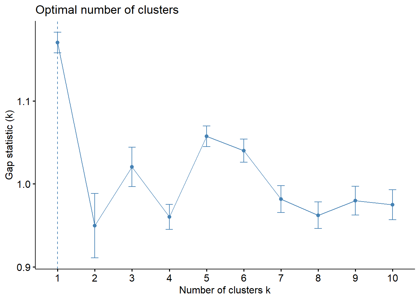
With reference to the gap statistic graph above, the recommended number of cluster to retain is 1. However, it is not logical to retain only one cluster. By examine the gap statistic graph, the 5-cluster gives the largest gap statistic and should be the next best cluster to pick.
Interpreting the dendrograms
plot(hclust_ward, cex = 0.6)
rect.hclust(hclust_ward,
            k = 5,
            border = 2:5)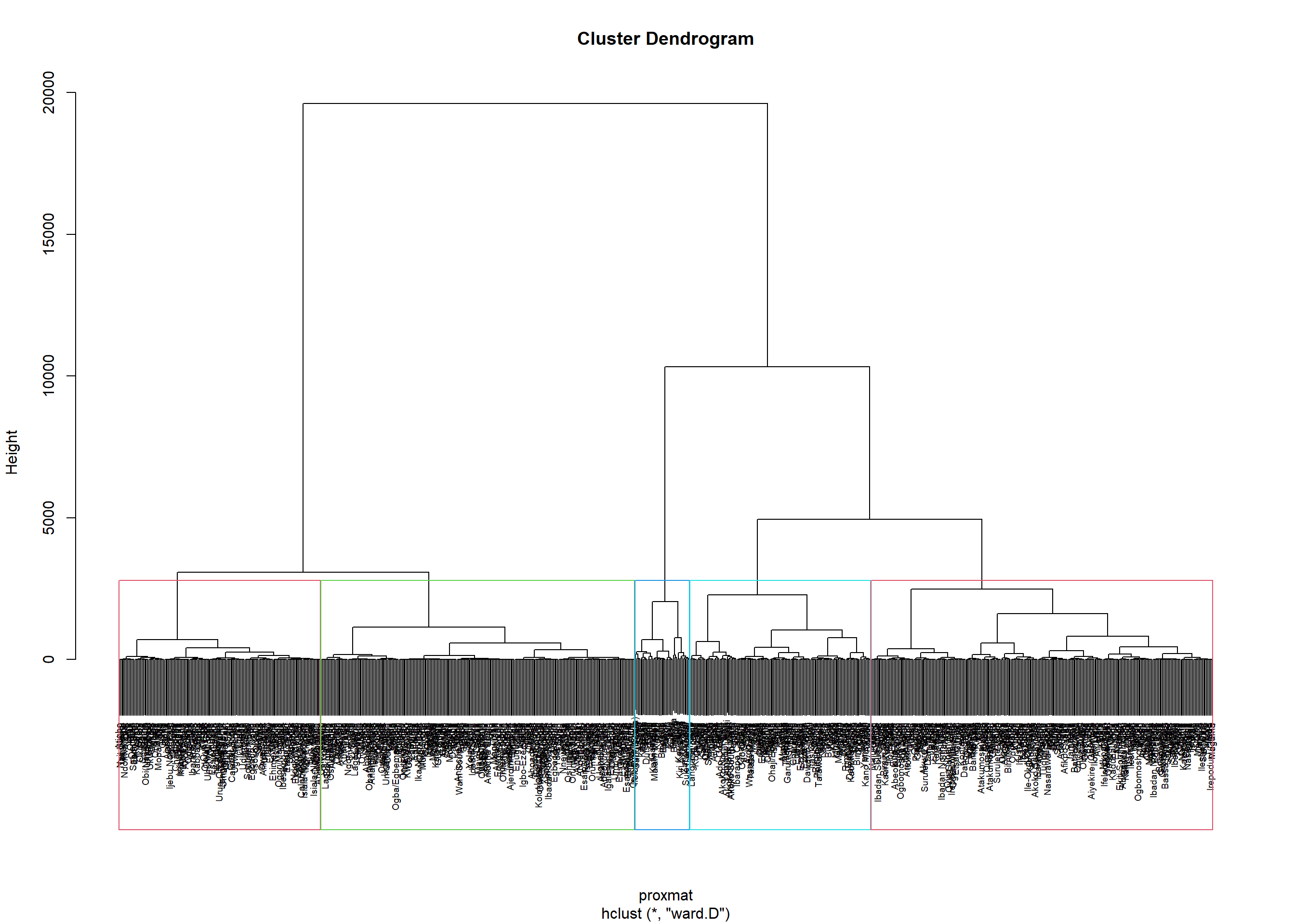
Visually-driven hierarchical clustering analysis
With heatmaply, we are able to build both highly interactive cluster heatmap or static cluster heatmap.
Transforming the data frame into a matrix
nga_wp_clu_mat <- data.matrix(nga_wp_clu)Plotting interactive cluster heatmap using heatmaply()
heatmaply(normalize(nga_wp_clu_mat),
          Colv=NA,
          dist_method = "euclidean",
          hclust_method = "ward.D",
          seriate = "OLO",
          colors = Blues,
          k_row = 5,
          margins = c(NA,200,60,NA),
          fontsize_row = 4,
          fontsize_col = 5,
          main="Geographic Segmentation of Nigeria by Water point indicators",
          xlab = "Water point indicators Indicators",
          ylab = "Shape Name of Nigeria"
          )
Mapping the clusters formed
groups <- as.factor(cutree(hclust_ward, k=5))nga_wp_cluster <- cbind(nga_wp, as.matrix(groups)) %>%
rename(`CLUSTER`=`as.matrix.groups.`)qtm(nga_wp_cluster, "CLUSTER")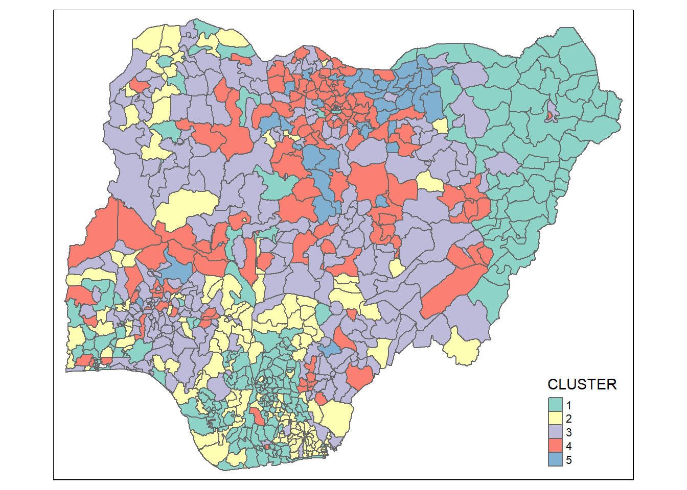
8 Spatially Constrained Clustering: SKATER approach
Converting into SpatialPolygonsDataFrame
First, I convert nga_wp into SpatialPolygonsDataFrame. This is because SKATER function only support sp objects such as SpatialPolygonDataFrame.
The code chunk below uses as_Spatial() of sf package to convert nga_wpinto a SpatialPolygonDataFrame called nga_sp.
nga_sp <- as_Spatial(nga_wp)Computing Neighbour List
nga.nb <- poly2nb(nga_sp,snap=1000)
summary(nga.nb)
Neighbour list object:
Number of regions: 774
Number of nonzero links: 4440
Percentage nonzero weights: 0.7411414
Average number of links: 5.736434
1 region with no links:
86
Link number distribution:
0 1 2 3 4 5 6 7 8 9 10 11 12 14
1 2 14 57 125 182 140 122 72 41 12 4 1 1
2 least connected regions:
138 560 with 1 link
1 most connected region:
508 with 14 linksplot(nga_sp,
border=grey(.5))
plot(nga.nb,
coordinates(nga_sp),
col="blue",
add=TRUE)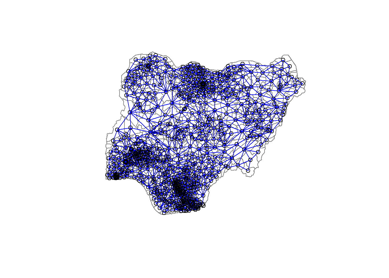
9 Spatially Constrained Clustering: ClustGeo Method
Ward-like hierarchical clustering: ClustGeo
To perform non-spatially constrained hierarchical clustering, we only need to provide the function a dissimilarity matrix as shown in the code chunk below
nongeo_cluster <- hclustgeo(proxmat)
plot(nongeo_cluster, cex = 0.5)
rect.hclust(nongeo_cluster,
            k = 5,
            border = 2:5)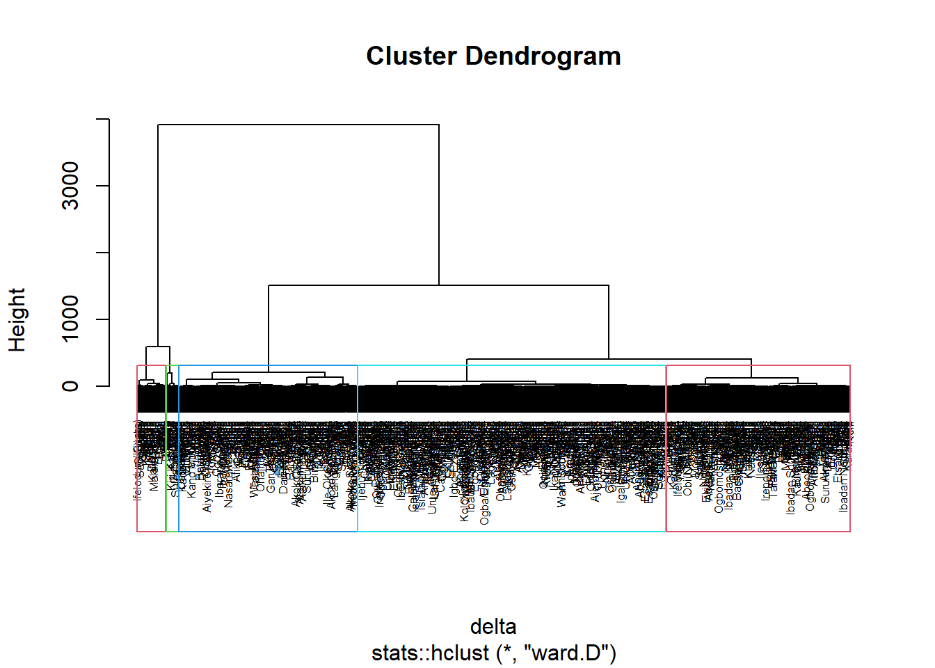
Mapping the clusters formed
groups <- as.factor(cutree(nongeo_cluster, k=5))nga_wp_ngeo_cluster <- cbind(nga_wp, as.matrix(groups)) %>%
rename(`CLUSTER` = `as.matrix.groups.`)qtm(nga_wp_ngeo_cluster, "CLUSTER")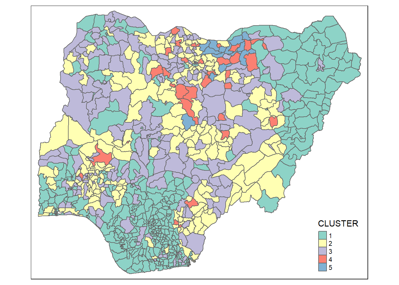
Spatially Constrained Hierarchical Clustering
Before we can performed spatially constrained hierarchical clustering, a spatial distance matrix will be derived by using st_distance() of sf package.
dist <- st_distance(nga_wp, nga_wp)
distmat <- as.dist(dist)
Notice that as.dist() is used to convert the data frame into matrix.
Next, choicealpha() will be used to determine a suitable value for the mixing parameter alpha as shown in the code chunk below.
cr <- choicealpha(proxmat, distmat, range.alpha = seq(0, 1, 0.1), K=5, graph = TRUE)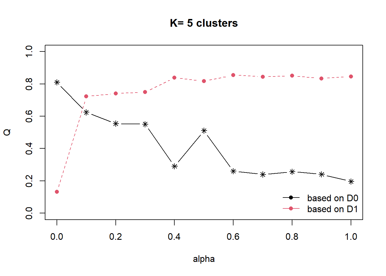
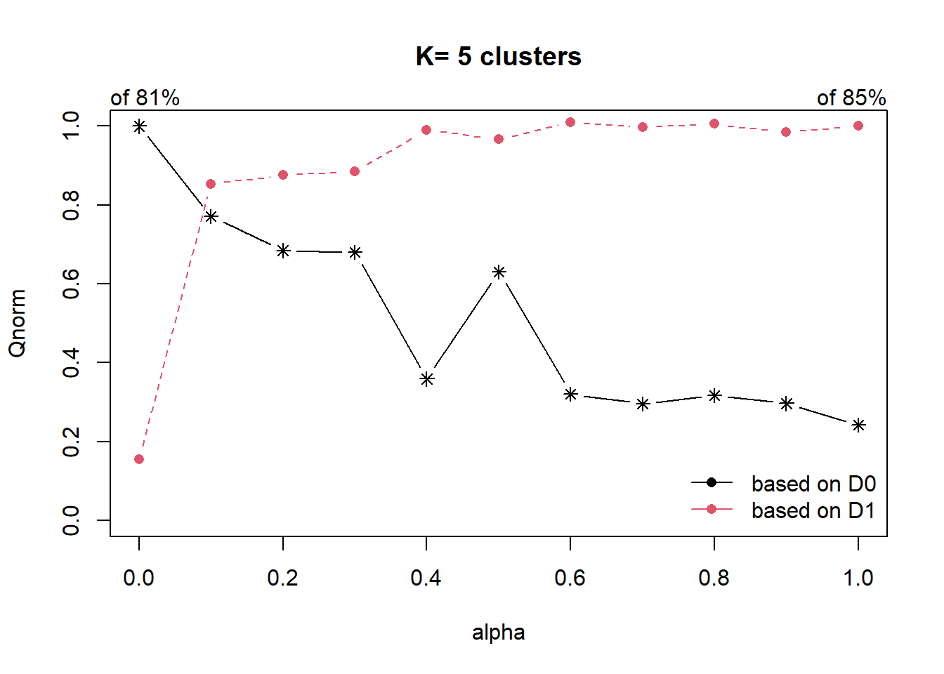
With reference to the graphs above, alpha = 0.1 will be used as shown in the code chunk below.
clustG <- hclustgeo(proxmat, distmat, alpha = 0.1)groups <- as.factor(cutree(clustG, k=5))nga_wp_Gcluster <- cbind(nga_wp, as.matrix(groups)) %>%
rename(`CLUSTER` = `as.matrix.groups.`)qtm(nga_wp_Gcluster, "CLUSTER")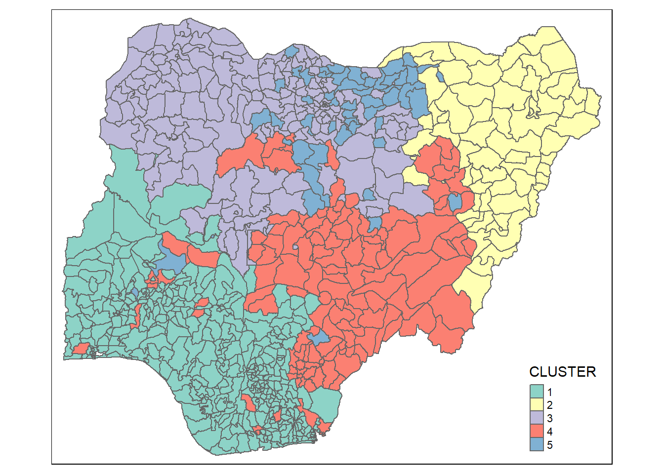
10 Visual Interpretation of Clusters
Multivariate Visualisation
Past studies shown that parallel coordinate plot can be used to reveal clustering variables by cluster very effectively. In the code chunk below, ggparcoord() of GGally package
ggparcoord(data = nga_wp_ngeo_cluster,
           columns = c(14:19),
           groupColumn = "CLUSTER",
           scale = "std",
           alphaLines = 0.2,
           boxplot = TRUE,
           title = "Multiple Parallel Coordinates Plots of water points Variables by Cluster") +
  facet_grid(~ CLUSTER) +
  theme(axis.text.x = element_text(angle = 30)) +
  scale_color_viridis(option = "D", discrete=TRUE)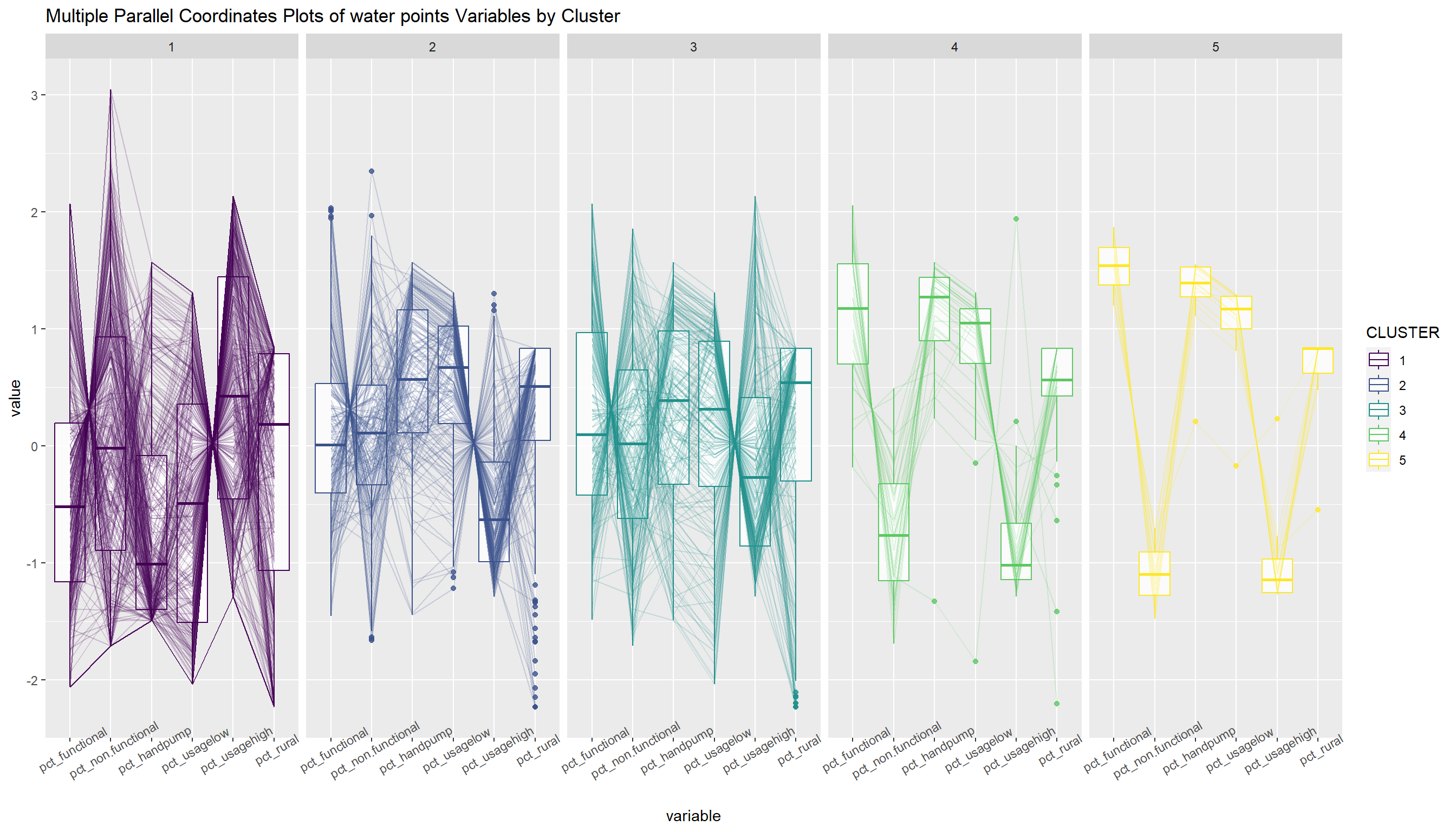
The parallel coordinate plot above reveals that
we can also compute the summary statistics such as mean, median, sd, etc to complement the visual interpretation.
In the code chunk below, group_by() and summarise() of dplyr are used to derive mean values of the clustering variables.
nga_wp_ngeo_cluster %>%
  st_set_geometry(NULL) %>%
  group_by(CLUSTER) %>%
  summarise(mean_pct_functional = mean(pct_functional),
            mean_pct_non.functional = mean(pct_non.functional),
            mean_pct_handpump = mean(pct_handpump),
            mean_pct_usagelow = mean(pct_usagelow),
            mean_pct_usagehigh = mean(pct_usagehigh),
            mean_pct_rural = mean(pct_rural))
# A tibble: 5 × 7
CLUSTER mean_pct_functional mean_pct_non.fun…¹ mean_…² mean_…³ mean_…⁴ mean_…⁵
<chr> <dbl> <dbl> <dbl> <dbl> <dbl> <dbl>
1 1 0.404 0.369 0.277 0.450 0.511 0.650
2 2 0.526 0.381 0.670 0.768 0.232 0.802
3 3 0.563 0.362 0.579 0.656 0.344 0.749
4 4 0.766 0.210 0.832 0.857 0.143 0.846
5 5 0.868 0.132 0.917 0.923 0.0772 0.945
# … with abbreviated variable names ¹mean_pct_non.functional,
# ²mean_pct_handpump, ³mean_pct_usagelow, ⁴mean_pct_usagehigh,
# ⁵mean_pct_ruralnga_wp_ngeo_cluster %>%
st_set_geometry(NULL) %>%
group_by(CLUSTER) %>%
summarise(median_pct_functional = median(pct_functional),
median_pct_non.functional = median(pct_non.functional),
median_pct_handpump = median(pct_handpump),
median_pct_usagelow = median(pct_usagelow),
median_pct_usagehigh = median(pct_usagehigh),
median_pct_rural = median(pct_rural))# A tibble: 5 × 7
CLUSTER median_pct_functional median_pct_non…¹ media…² media…³ media…⁴ media…⁵
<chr> <dbl> <dbl> <dbl> <dbl> <dbl> <dbl>
1 1 0.373 0.356 0.158 0.462 0.5 0.788
2 2 0.501 0.383 0.674 0.808 0.192 0.893
3 3 0.522 0.363 0.614 0.703 0.297 0.904
4 4 0.783 0.199 0.904 0.922 0.0782 0.912
5 5 0.872 0.128 0.943 0.958 0.0421 1
# … with abbreviated variable names ¹median_pct_non.functional,
# ²median_pct_handpump, ³median_pct_usagelow, ⁴median_pct_usagehigh,
# ⁵median_pct_ruralnga_wp_ngeo_cluster %>%
st_set_geometry(NULL) %>%
group_by(CLUSTER) %>%
summarise(sd_pct_functional = sd(pct_functional),
sd_pct_non.functional = sd(pct_non.functional),
sd_pct_handpump = sd(pct_handpump),
sd_pct_usagelow = sd(pct_usagelow),
sd_pct_usagehigh = sd(pct_usagehigh),
sd_pct_rural = sd(pct_rural))# A tibble: 5 × 7
CLUSTER sd_pct_functional sd_pct_non.functio…¹ sd_pc…² sd_pc…³ sd_pc…⁴ sd_pc…⁵
<chr> <dbl> <dbl> <dbl> <dbl> <dbl> <dbl>
1 1 0.253 0.249 0.295 0.307 0.311 0.357
2 2 0.183 0.156 0.217 0.180 0.180 0.256
3 3 0.208 0.184 0.263 0.256 0.256 0.326
4 4 0.148 0.123 0.193 0.186 0.186 0.230
5 5 0.0544 0.0544 0.114 0.115 0.115 0.121
# … with abbreviated variable names ¹sd_pct_non.functional, ²sd_pct_handpump,
# ³sd_pct_usagelow, ⁴sd_pct_usagehigh, ⁵sd_pct_rural